library(tidyverse)
library(glue)

library(gt)

library(hrbrthemes)
library(ggpomological)

library(highcharter)
Grab the the most recent advanced metrics from basketball reference using the {nbastatR} package by Alex Bresler. Note, running bref_players_stats() will assign the output data frames, dataBREFPlayerTotals and dataBREFPlayerAdvanced, to the environment, so we don’t need to do anything else (I rename them for my own sanity).
library(nbastatR)
bref_players_stats(seasons = 2019, tables = c("advanced", "totals"),
                   widen = TRUE, assign_to_environment = TRUE)
bref_advanced <- dataBREFPlayerAdvanced
bref_totals <- dataBREFPlayerTotals
I always like to start out by skimming with the skimr package…
skimr::skim(bref_advanced)
#> Skim summary statistics
#>  n obs: 501
#>  n variables: 36
#>
#> ── Variable type:character ──────────────────────────────────────────────────────────────────
#>            variable missing complete   n min max empty n_unique
#>            idPlayer       0      501 501   6   9     0      501
#>      idPlayerSeason       0      501 501  11  14     0      501
#>          idPosition       0      501 501   1   5     0       13
#>          namePlayer       0      501 501   4  24     0      501
#>      namePlayerBREF       0      501 501   7  24     0      501
#>          slugSeason       0      501 501   7   7     0        1
#>        slugTeamBREF       0      501 501   3   3     0       31
#>   urlPlayerHeadshot      15      486 501  86  89     0      486
#>  urlPlayerThumbnail       0      501 501  52  89     0      501
#>
#> ── Variable type:logical ────────────────────────────────────────────────────────────────────
#>     variable missing complete   n mean           count
#>  isHOFPlayer       0      501 501    0 FAL: 501, NA: 0
#>
#> ── Variable type:numeric ────────────────────────────────────────────────────────────────────
#>         variable missing complete   n       mean         sd      p0
#>        agePlayer       0      501 501     26.08       4.18    19
#>       countGames       0      501 501     44.04      22.57     1
#>      idPlayerNBA       0      501 501 880176.29  724825.17  1114
#>          minutes       0      501 501   1005.99     745.5      1
#>        pct3PRate       5      496 501      0.36       0.21     0
#>           pctAST       0      501 501      0.13       0.094    0
#>           pctBLK       0      501 501      0.17       0.28     0
#>           pctDRB       0      501 501      0.15       0.084    0
#>        pctFTRate       5      496 501      0.24       0.14     0
#>           pctORB       0      501 501      0.073      0.14     0
#>           pctSTL       0      501 501      0.12       0.26     0
#>           pctTOV       4      497 501      0.12       0.055    0
#>           pctTRB       0      501 501      0.1        0.059    0
#>  pctTrueShooting       4      497 501      0.53       0.11     0
#>           pctUSG       0      501 501      0.19       0.059    0
#>         ratioBPM       0      501 501     -1.95       5.61   -52.7
#>        ratioDBPM       0      501 501     -0.55       2.68   -20.5
#>         ratioDWS       0      501 501      1.02       0.98    -0.4
#>        ratioOBPM       0      501 501     -1.4        4.3    -36.1
#>         ratioOWS       0      501 501      1.1        1.66    -2.7
#>         ratioPER       0      501 501     12.99       7.62   -38
#>        ratioVORP       0      501 501      0.51       1.18    -1.9
#>          ratioWS       0      501 501      2.12       2.44    -1.6
#>     ratioWSPer48       0      501 501      0.076      0.12    -0.95
#>       yearSeason       0      501 501   2018          0     2018
#>  yearSeasonFirst      15      486 501   2013.49       4.36  1989
#>        p25       p50         p75       p100     hist
#>     23        25          29          42    ▃▇▇▆▃▁▁▁
#>     26        50          64          72    ▃▂▂▂▂▃▅▇
#>  2e+05     2e+05     1628383     1629541    ▇▁▁▁▁▁▁▇
#>    292       945        1672        2671    ▇▃▃▃▃▃▃▁
#>      0.23      0.38        0.52        0.9  ▇▃▇▇▇▅▂▁
#>      0.068     0.11        0.18        0.59 ▆▇▃▂▁▁▁▁
#>      0.012     0.024       0.2         0.9  ▇▁▁▁▁▁▁▁
#>      0.1       0.14        0.19        0.92 ▅▇▂▁▁▁▁▁
#>      0.15      0.23        0.32        0.86 ▃▇▇▃▂▁▁▁
#>      0.02      0.034       0.074       1    ▇▁▁▁▁▁▁▁
#>      0.013     0.016       0.024       0.9  ▇▁▁▁▁▁▁▁
#>      0.095     0.12        0.15        0.5  ▂▇▆▁▁▁▁▁
#>      0.062     0.087       0.13        0.52 ▅▇▃▁▁▁▁▁
#>      0.5       0.55        0.58        0.83 ▁▁▁▁▃▇▁▁
#>      0.15      0.18        0.22        0.47 ▁▁▇▆▂▁▁▁
#>     -3.9      -1.4         0.6        27.2  ▁▁▁▁▃▇▁▁
#>     -1.7      -0.5         0.9         8.6  ▁▁▁▁▂▇▂▁
#>      0.2       0.8         1.5         5    ▇▇▆▃▂▁▁▁
#>     -2.8      -1.1         0.3        22.3  ▁▁▁▁▇▂▁▁
#>      0         0.5         1.7         9.1  ▁▇▆▂▂▁▁▁
#>      9.4      12.6        16.5        80.8  ▁▁▁▇▁▁▁▁
#>     -0.1       0.1         0.8         8.1  ▁▇▂▁▁▁▁▁
#>      0.2       1.3         3.1        13    ▆▇▅▂▁▁▁▁
#>      0.039     0.081       0.13        1.26 ▁▁▁▇▂▁▁▁
#>   2018      2018        2018        2018    ▁▁▁▇▁▁▁▁
#>   2011      2015        2017        2018    ▁▁▁▁▁▂▃▇
Now we can filter and munge as needed:
adv_player_stats <- bref_advanced %>%
  filter(minutes >= 500) %>%
  mutate(bref_url = glue::glue("https://www.basketball-reference.com/players/{stringr::str_sub(idPlayer, 1, 1)}/{idPlayer}.html"),
         bref_link = glue::glue('<a href="{bref_url}">{namePlayer}</a>'))
Collapse positions into front and backcourt:
unique_positions <- unique(bref_advanced$idPosition)
frontcourt <- c("PF", "SF", "C", "PF-SF", "C-PF", "SG-PF", "SF-PF")
backcourt <- c("PG", "SG", "PG-SG", "SG-PG", "SF-SG", "SG-SF")

bref_efg <- bref_totals %>%
  select(one_of(c("idPlayer", "pctEFG")))

adv_player_stats <- adv_player_stats %>%
  left_join(bref_efg, by = "idPlayer") %>%
  mutate( "position" = case_when(
    idPosition %in% frontcourt ~ "frontcourt",
    idPosition %in% backcourt ~ "backcourt",
    TRUE ~ "other"),
    "position" = as.factor(position)
  )
Let’s also get some info from the NBA Stats API using teams_players_states(). By using assign_to_environment = TRUE, we’ll automatically get a data frame dataGeneralPlayers. For now I just want players’ offensive rating1, ortg, and defensive rating2, drtg.
nbastatR::teams_players_stats(seasons = 2019, types = c("player"),
                              tables = "general", measures = "Advanced",
                              assign_to_environment = TRUE)
player_rtgs <- dataGeneralPlayers %>%
  select(one_of(c("idPlayer", "ortg", "drtg")))

adv_player_stats <- adv_player_stats %>%
  left_join(player_rtgs, by = c("idPlayerNBA" = "idPlayer"))
adv_player_stats %>%
  ggplot(aes(x = ratioPER)) +
  geom_histogram()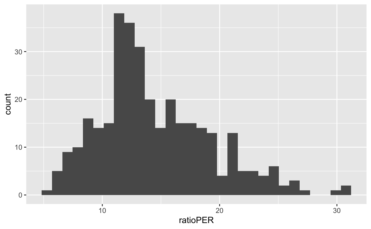
Let’s get some help from glue and hrbrthemes…
adv_player_stats %>%
  ggplot(aes(x = ratioPER)) +
  geom_histogram(alpha = 0.7, fill = "#011627") +
  labs(title = "PER for players with 500+ minutes",
       subtitle = "NBA 2018-2019 season",
       caption = glue::glue("data via nbastatR {yesterday}")) +
  hrbrthemes::theme_ipsum_rc()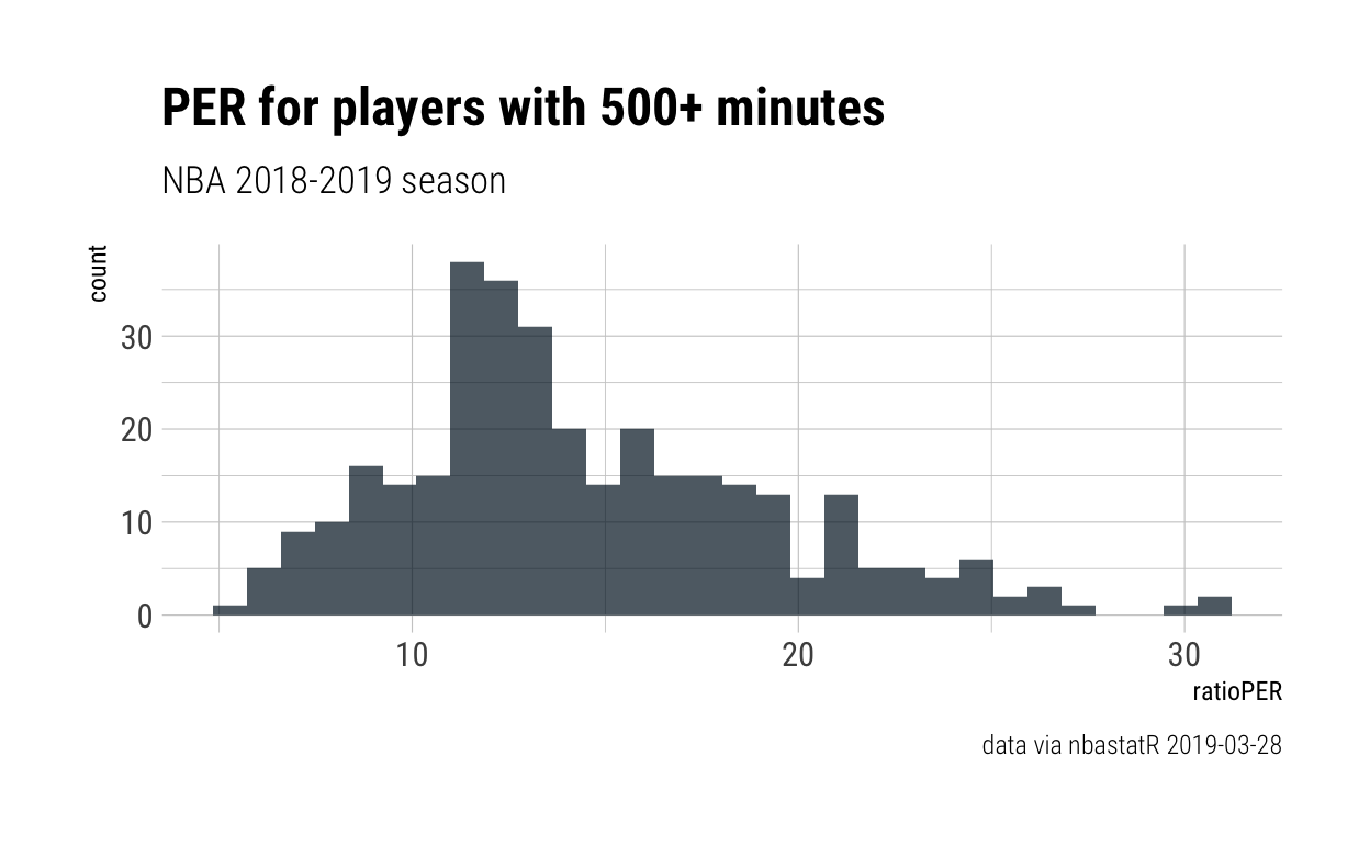
adv_player_stats %>%
  ggplot(aes(x = ratioVORP)) +
  geom_histogram(alpha = 0.7, fill = "#011627") +
  labs(title = "Value Over Replacement Player (VORP)",
       subtitle = "NBA 2018-2019 season, players with 500+ minutes",
       caption = glue::glue("data via nbastatR {yesterday}")) +
  hrbrthemes::theme_ipsum_rc()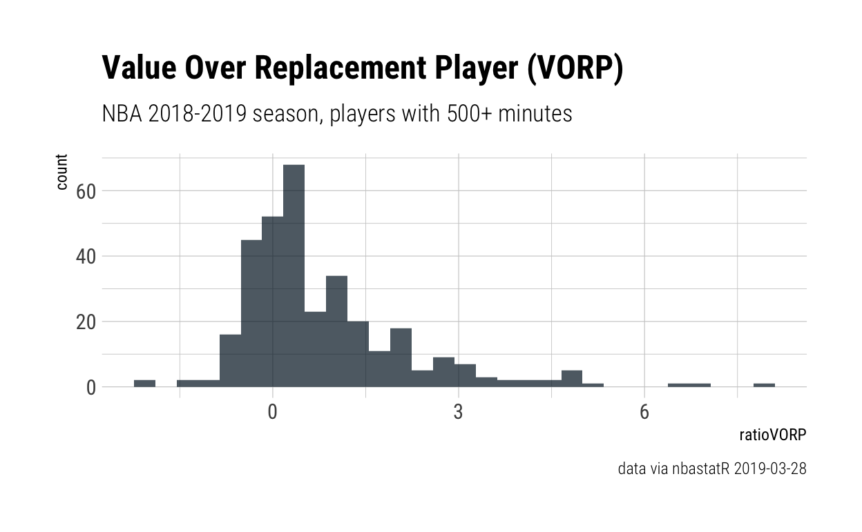
adv_player_stats %>%
  ggplot(aes(x = ratioWS)) +
  geom_histogram(alpha = 0.7, fill = "#011627") +
  labs(title = "Win Shares for players with 500+ minutes",
       subtitle = "NBA 2018-2019 season",
       caption = glue::glue("data via nbastatR {yesterday}")) +
  hrbrthemes::theme_ipsum_rc()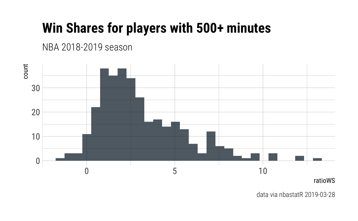
Histograms are all well and good, but let’s look at something a little more interesting…
adv_player_stats %>%
  ggplot(aes(x = ratioOBPM, y = ratioDBPM)) +
  geom_point() +
  geom_hline(yintercept = 0, alpha = 0.6, lty = "dashed") +
  geom_vline(xintercept = 0, alpha = 0.6, lty = "dashed") +
  labs(title = "Offensive vs. Defensive Box Plus-Minus",
       subtitle = glue::glue("NBA 2018-2019 season through {yesterday}"),
       caption = glue::glue("data via nbastatR"),
       x = "OBPM",
       y = "DBPM") +
  hrbrthemes::theme_ipsum_rc()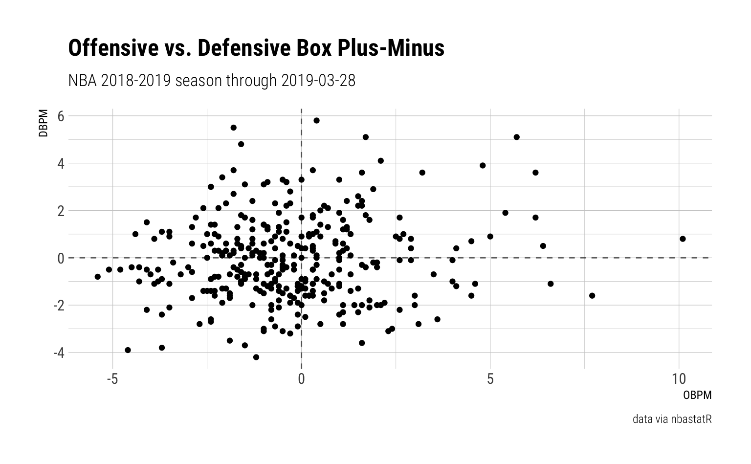
Things are a pretty boring without annotation — and we’re not doing much in the way of storytelling. Luckily Hiroaki Yutani’s gghighlight package can help us out with that!
Because gghighlight uses a predicate function to determine what to highlight, I’ll make a little helper fun to get the top 10 players for some variable.
get_top10 <- function(df, column) {
  require(rlang)
  column <- enquo(column)
  dplyr::top_n(df, n = 10, wt = !!column) %>%
    pull(namePlayer)
}
Things are looking a little more complex, so let’s look at the pieces of code in this next section.
# get top 10 for desired variable (in this case ratioBPM)
top10_BPM <- top_n(adv_player_stats, n = 10, wt = ratioBPM) %>%
  pull(namePlayer)

adv_player_stats %>%
  ggplot(aes(x = ratioOBPM, y = ratioDBPM)) +
  geom_point(color = "#011627") +
  gghighlight::gghighlight(namePlayer %in% top10_BPM, label_key = namePlayer,
                           label_params = list(fill = ggplot2::alpha("white", 0.8),
                                                 box.padding = 0,
                                                 family = "Roboto Condensed"),
                           unhighlighted_colour = "#007190") +
  geom_hline(yintercept = 0, alpha = 0.6, lty = "dashed") +
  geom_vline(xintercept = 0, alpha = 0.6, lty = "dashed") +
  labs(title = "Offensive vs. Defensive Box Plus-Minus: Top 10 Box Plus/Minus",
       subtitle = glue::glue("NBA 2018-2019 season through {yesterday}"),
       caption = glue::glue("data via nbastatR"),
       x = "OBPM",
       y = "DBPM") +
  hrbrthemes::theme_ipsum_rc()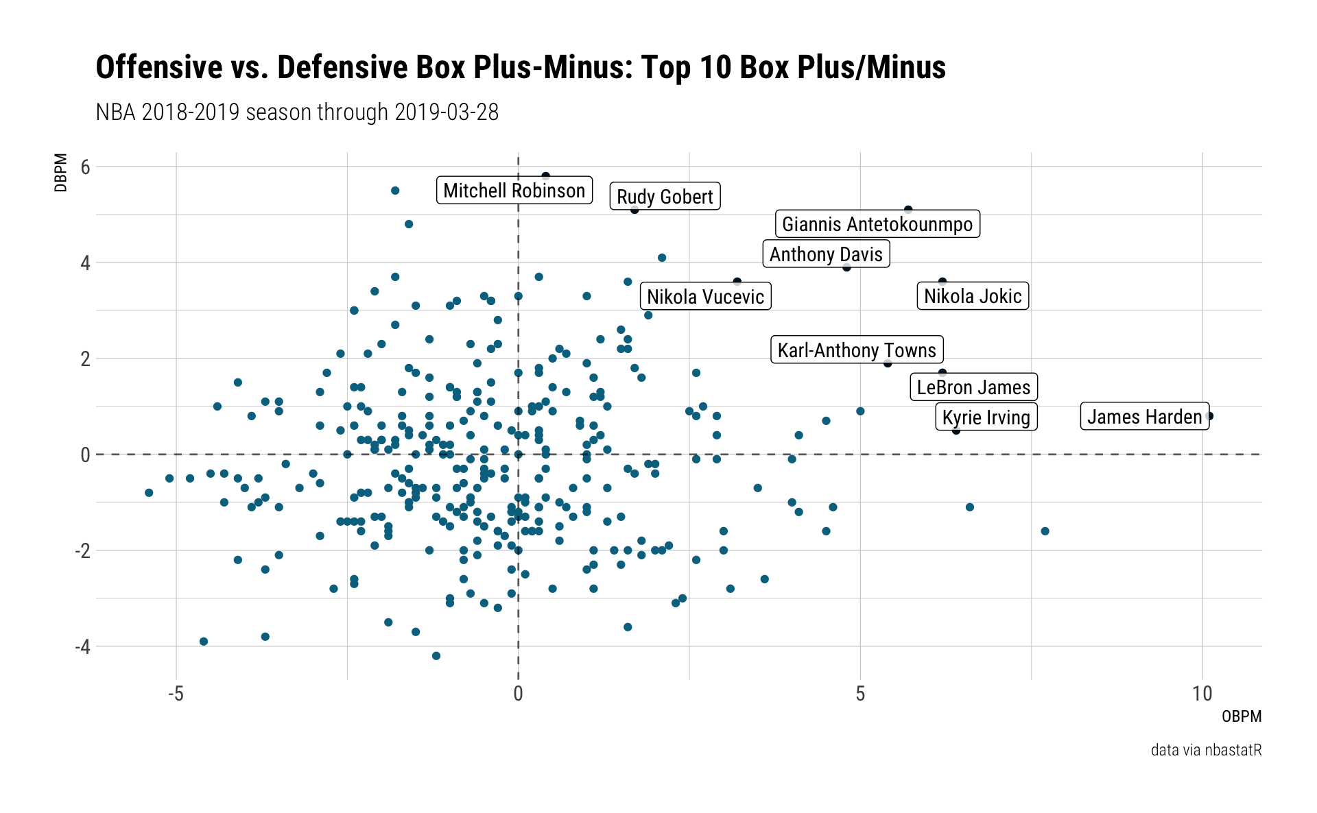
Predicate functions won’t always hit everything you want to see, which is why interactive visualizations can be a great tool for exploration. There are also some widgets and add-ins in RStudio that can help out with this.3
Since we’re using distill for R Markdown, we have some nice options in terms of figure layout. Below, I’ll use layout="l-body-outset" as a chunk parameter.
top10_WS <- get_top10(adv_player_stats, ratioWSPer48)

adv_player_stats %>%
  ggplot(aes(x = ratioOWS, y = ratioDWS)) +
  geom_point(color = "#011627") +
  gghighlight::gghighlight(namePlayer %in% top10_WS, label_key = namePlayer,
                           label_params = list(fill = ggplot2::alpha("white", 0.8),
                                                 box.padding = 0,
                                                 family = "Roboto Condensed"),
                           unhighlighted_colour = "#007190") +
  geom_hline(yintercept = 0, alpha = 0.6, lty = "dashed") +
  geom_vline(xintercept = 0, alpha = 0.6, lty = "dashed") +
  labs(title = "Offensive vs. Defensive Win Shares: Top 10 WS Per 48",
       subtitle = glue::glue("NBA 2018-2019 season through {yesterday}"),
       caption = glue::glue("data via nbastatR"),
       x = "OWS",
       y = "DWS") +
  hrbrthemes::theme_ipsum_rc()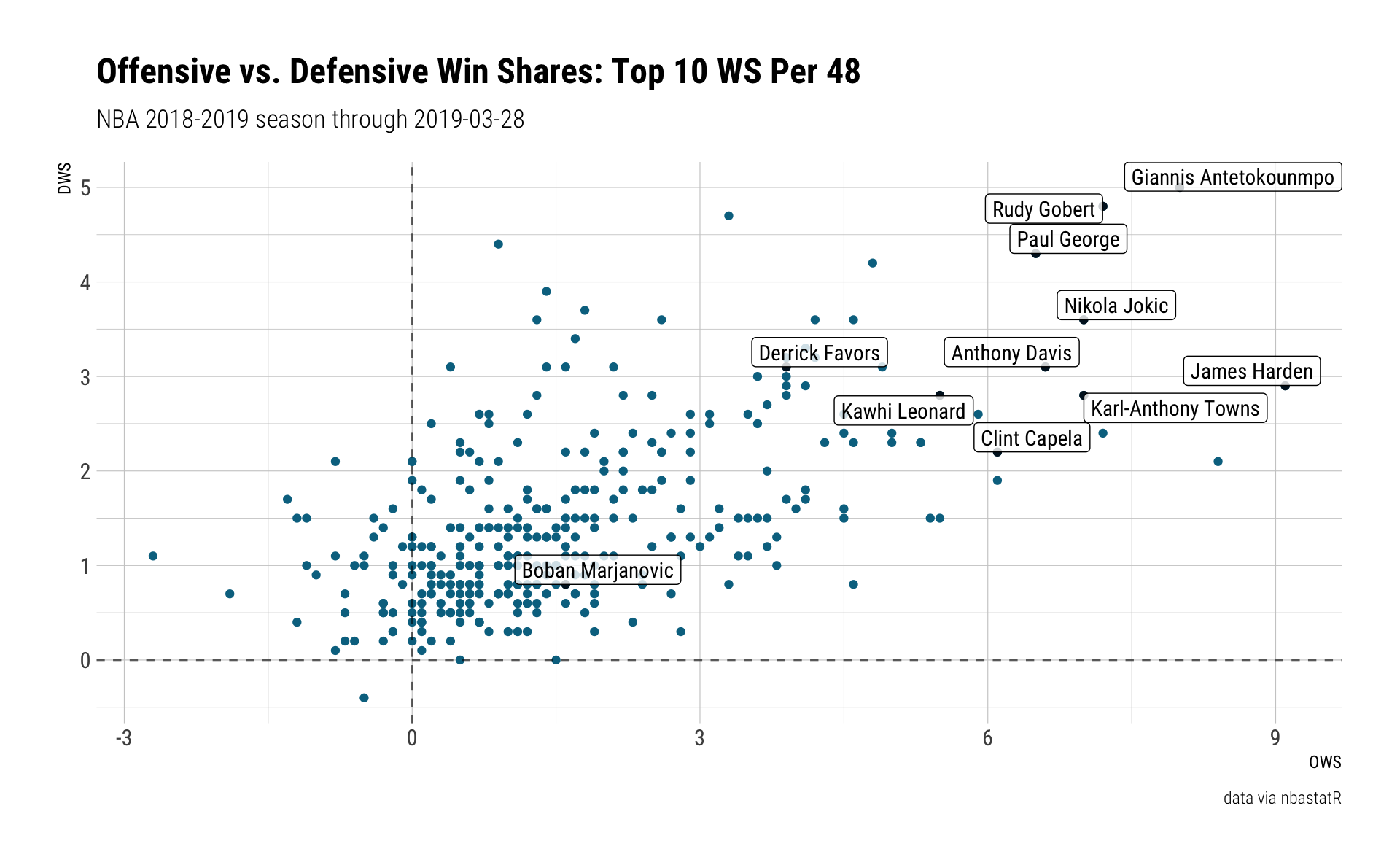
We can go even wider by using layout="l-page".
top10_EFG <- get_top10(adv_player_stats, pctEFG)

adv_player_stats %>%
  ggplot(aes(x = (pctTrueShooting - mean(pctTrueShooting)), y = (ratioPER - mean(ratioPER)))) +
  geom_point(color = "#011627") +
  gghighlight::gghighlight(namePlayer %in% top10_EFG, label_key = namePlayer,
                           label_params = list(fill = ggplot2::alpha("white", 0.8),
                                                 box.padding = 0,
                                                 family = "Roboto Condensed"),
                           unhighlighted_colour = "#007190") +
  geom_hline(yintercept = 0, alpha = 0.6, lty = "dashed") +
  geom_vline(xintercept = 0, alpha = 0.6, lty = "dashed") +
  labs(title = "TS% above avg vs. PER above avg: Top 10 EFG%",
       subtitle = glue::glue("NBA 2018-2019 season"),
       caption = glue::glue("data via nbastatR, {yesterday}"),
       x = "true shooting %",
       y = "player efficiency rating") +
  hrbrthemes::theme_ipsum_rc()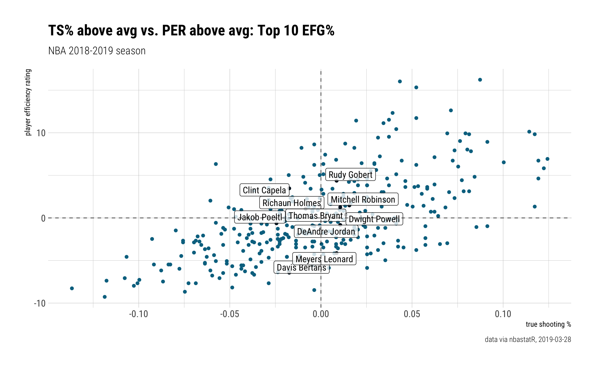
Piping through the grammar of tables…
One of my latest favorite packages to play with is Rich Iannone’s {gt}:
adv_player_stats %>%
  select(namePlayer, ratioBPM, ratioOBPM, ratioDBPM, bref_url, urlPlayerThumbnail) %>%
  arrange(desc(ratioBPM)) %>%
  top_n(n = 10, wt = ratioBPM) %>%
  gt::gt(rowname_col = "namePlayer") %>%
  tab_header(
    title = md("**Top 10 Box Plus/Minus**")
  ) %>%
  cols_label(
    ratioBPM = md("**BPM**"),
    ratioOBPM = md("**OBPM**"),
    ratioDBPM = md("**DBPM**"),
    bref_url = md("**Link**"),
    urlPlayerThumbnail = md("")
  ) %>%
  text_transform(
    locations = cells_data(vars(bref_url)),
    fn = function(x) {
      sprintf("<a href=%s>profile</a>", x)
    }
  ) %>%
    text_transform(
    locations = cells_data(vars(urlPlayerThumbnail)),
    fn = function(x) {
      web_image(url = x)
    }
  ) %>%
  tab_source_note(
    md("source: [basketball-reference.com](https://www.basketball-reference.com) via [nbastatR](http://asbcllc.com/nbastatR/index.html)")
  ) %>%
  tab_footnote(
    footnote = ("Players with 500+ minutes."),
    locations = cells_title("title")
    ) %>%
  tab_footnote(
    footnote = ("Box Plus/Minus: a box score estimate of the points per 100 possessions that a player contributed above a league-average player, translated to an average team."),
    locations = cells_column_labels(
      columns = vars(ratioBPM)
    )
  ) %>%
  tab_footnote(
    footnote = ("Offensive Box Plus/Minus."),
    locations = cells_column_labels(
      columns = vars(ratioOBPM)
    )
  ) %>%
  tab_footnote(
    footnote = ("Defensive Box Plus/Minus."),
    locations = cells_column_labels(
      columns = vars(ratioDBPM)
    )
  ) %>%
  tab_options(footnote.glyph = c("*, †, ‡, §, ¶, ‖"),
table.width = px(640))| Top 10 Box Plus/Minus* | ||||||
|---|---|---|---|---|---|---|
| BPM † | OBPM ‡ | DBPM § | Link | |||
| James Harden | 11.0 | 10.1 | 0.8 | profile |  |
|
| Giannis Antetokounmpo | 10.8 | 5.7 | 5.1 | profile |  |
|
| Nikola Jokic | 9.8 | 6.2 | 3.6 | profile |  |
|
| Anthony Davis | 8.7 | 4.8 | 3.9 | profile |  |
|
| LeBron James | 7.9 | 6.2 | 1.7 | profile |  |
|
| Karl-Anthony Towns | 7.3 | 5.4 | 1.9 | profile |  |
|
| Kyrie Irving | 6.8 | 6.4 | 0.5 | profile |  |
|
| Nikola Vucevic | 6.8 | 3.2 | 3.6 | profile |  |
|
| Rudy Gobert | 6.8 | 1.7 | 5.1 | profile |  |
|
| Mitchell Robinson | 6.2 | 0.4 | 5.8 | profile |  |
|
| source: basketball-reference.com via nbastatR | ||||||
| * Players with 500+ minutes. † Box Plus/Minus: a box score estimate of the points per 100 possessions that a player contributed above a league-average player, translated to an average team. ‡ Offensive Box Plus/Minus. § Defensive Box Plus/Minus. |
||||||
adv_player_stats %>%
  select(urlPlayerHeadshot, namePlayer, ratioBPM, ratioOBPM, ratioDBPM) %>%
  arrange(desc(ratioOBPM)) %>%
  top_n(n = 10, wt = ratioOBPM) %>%
  gt::gt() %>%
  tab_header(
    title = md("**Top 10 Offensive Box Plus/Minus**")
  ) %>%
  cols_label(
    namePlayer = md("**Player**"),
    urlPlayerHeadshot = md(""),
    ratioBPM = md("**BPM**"),
    ratioOBPM = md("**OBPM**"),
    ratioDBPM = md("**DBPM**")
  ) %>%
    text_transform(
    locations = cells_data(vars(urlPlayerHeadshot)),
    fn = function(x) {
      web_image(url = x)
    }
  ) %>%
  tab_source_note(
    md("source: [basketball-reference.com](https://www.basketball-reference.com) via [nbastatR](http://asbcllc.com/nbastatR/index.html)")
  ) %>%
  tab_footnote(
    footnote = ("Players with 500+ minutes."),
    locations = cells_title("title")
  ) %>%
  tab_footnote(
    footnote = ("Box Plus/Minus; a box score estimate of the points per 100 possessions that a player contributed above a league-average player, translated to an average team."),
    locations = cells_column_labels(
      columns = vars(ratioBPM)
    )
  ) %>%
  tab_footnote(
    footnote = ("Offensive Box Plus/Minus."),
    locations = cells_column_labels(
      columns = vars(ratioOBPM)
    )
  ) %>%
  tab_footnote(
    footnote = ("Defensive Box Plus/Minus."),
    locations = cells_column_labels(
      columns = vars(ratioDBPM)
    )
  ) %>%
  tab_options(footnote.glyph = c("*, †, ‡, §, ¶, ‖"),
table.width = px(640))| Top 10 Offensive Box Plus/Minus* | |||||
|---|---|---|---|---|---|
| Player | BPM † | OBPM ‡ | DBPM § | ||
 |
James Harden | 11.0 | 10.1 | 0.8 | |
 |
Stephen Curry | 6.0 | 7.7 | -1.6 | |
 |
Damian Lillard | 5.5 | 6.6 | -1.1 | |
 |
Kyrie Irving | 6.8 | 6.4 | 0.5 | |
 |
LeBron James | 7.9 | 6.2 | 1.7 | |
 |
Nikola Jokic | 9.8 | 6.2 | 3.6 | |
 |
Giannis Antetokounmpo | 10.8 | 5.7 | 5.1 | |
 |
Karl-Anthony Towns | 7.3 | 5.4 | 1.9 | |
 |
Paul George | 5.8 | 5.0 | 0.9 | |
 |
Anthony Davis | 8.7 | 4.8 | 3.9 | |
| source: basketball-reference.com via nbastatR | |||||
| * Players with 500+ minutes. † Box Plus/Minus; a box score estimate of the points per 100 possessions that a player contributed above a league-average player, translated to an average team. ‡ Offensive Box Plus/Minus. § Defensive Box Plus/Minus. |
|||||
adv_player_stats %>%
  select(namePlayer, ratioBPM, ratioOBPM, ratioDBPM) %>%
  arrange(desc(ratioDBPM)) %>%
  top_n(n = 10, wt = ratioDBPM) %>%
  gt::gt() %>%
  tab_header(
    title = md("**Top 10 Defensive Box Plus/Minus**")
  ) %>%
  cols_label(
    namePlayer = md("**Player**"),
    ratioBPM = md("**BPM**"),
    ratioOBPM = md("**OBPM**"),
    ratioDBPM = md("**DBPM**")
  ) %>%
  tab_source_note(
    md("source: [basketball-reference.com](https://www.basketball-reference.com) via [nbastatR](http://asbcllc.com/nbastatR/index.html)")
  ) %>%
  tab_footnote(
    footnote = ("Players with 500+ minutes."),
    locations = cells_title("title")
  ) %>%
  tab_footnote(
    footnote = ("Box Plus/Minus; a box score estimate of the points per 100 possessions that a player contributed above a league-average player, translated to an average team."),
    locations = cells_column_labels(
      columns = vars(ratioBPM)
    )
  ) %>%
  tab_footnote(
    footnote = ("Offensive Box Plus/Minus."),
    locations = cells_column_labels(
      columns = vars(ratioOBPM)
    )
  ) %>%
  tab_footnote(
    footnote = ("Defensive Box Plus/Minus."),
    locations = cells_column_labels(
      columns = vars(ratioDBPM)
    )
  ) %>%
  tab_options(footnote.glyph = c("*, †, ‡, §, ¶, ‖"),
table.width = px(640))| Top 10 Defensive Box Plus/Minus* | ||||
|---|---|---|---|---|
| Player | BPM † | OBPM ‡ | DBPM § | |
| Mitchell Robinson | 6.2 | 0.4 | 5.8 | |
| Nerlens Noel | 3.8 | -1.8 | 5.5 | |
| Giannis Antetokounmpo | 10.8 | 5.7 | 5.1 | |
| Rudy Gobert | 6.8 | 1.7 | 5.1 | |
| Myles Turner | 3.2 | -1.6 | 4.8 | |
| Russell Westbrook | 6.1 | 2.1 | 4.1 | |
| Anthony Davis | 8.7 | 4.8 | 3.9 | |
| Joakim Noah | 1.9 | -1.8 | 3.7 | |
| Mason Plumlee | 4.0 | 0.3 | 3.7 | |
| Jusuf Nurkic | 5.2 | 1.6 | 3.6 | |
| Nikola Jokic | 9.8 | 6.2 | 3.6 | |
| Nikola Vucevic | 6.8 | 3.2 | 3.6 | |
| source: basketball-reference.com via nbastatR | ||||
| * Players with 500+ minutes. † Box Plus/Minus; a box score estimate of the points per 100 possessions that a player contributed above a league-average player, translated to an average team. ‡ Offensive Box Plus/Minus. § Defensive Box Plus/Minus. |
||||
Highcharts
Messing around with highcharts courtesy of Joshua Kunst’s {highcharter} package.
library(highcharter)
hchart(adv_player_stats, "scatter", hcaes(x = "ratioOBPM", y = "ratioDBPM", group = "position", name = "namePlayer", OBPM = "ratioOBPM", DBPM = "ratioDBPM", position = "position")) %>%
  hc_tooltip(pointFormat = "<b>{point.name}</b><br />OBPM: {point.OBPM}<br />DBPM: {point.DBPM}") %>%
  hc_title(text = "Offensive vs. Defensive Box Plus/Minus") %>%
  hc_subtitle(text = "NBA 2018-2019 Season") %>%
  hc_credits(enabled = TRUE,
             text = "data via nbastatR",
             style = list(
               fontSize = "10px"
               )
             ) %>%
  hc_add_theme(hc_theme_538())
hchart(adv_player_stats, "scatter", hcaes(x = "ratioOWS", y = "ratioDWS", group = "position", name = "namePlayer", OWS = "ratioOWS", DWS = "ratioDWS", position = "position")) %>%
  hc_tooltip(pointFormat = "<b>{point.name}</b><br />OWS: {point.OWS}<br />DWS: {point.DWS}") %>%
  hc_title(text = "Offensive vs. Defensive Win Shares") %>%
  hc_subtitle(text = "NBA 2018-2019 Season") %>%
  hc_credits(enabled = TRUE,
             text = "data via nbastatR",
             style = list(
               fontSize = "10px"
               )
             ) %>%
  hc_add_theme(hc_theme_economist())
hchart(adv_player_stats, "scatter",
       hcaes(x = "pctTrueShooting", y = "ratioPER",
             name = "namePlayer", TS = "pctTrueShooting",
             PER = "ratioPER", position = "position")) %>%
  hc_tooltip(pointFormat = "<b>{point.name}</b><br />TS%: {point.TS}<br />PER: {point.PER}<br />Position: {point.position}") %>%
  hc_title(text = "True Shooting % vs Player Efficiency Rating") %>%
  hc_subtitle(text = "NBA 2018-2019 Season") %>%
  hc_credits(enabled = TRUE,
             text = "data via nbastatR",
             style = list(
               fontSize = "14px"
               )
             ) %>%
  hc_add_theme(hc_theme_chalk(
    plotOptions = list(
      scatter = list(
        marker = list(radius = 4,
                      fillOpacity = 0.3) # actually this does nothing
        )
      )
    )
  )
hc <- hchart(adv_player_stats, "scatter", hcaes(x = "ratioOWS", y = "ratioDWS", group = "position", name = "namePlayer", OWS = "ratioOWS", DWS = "ratioDWS", Position = "position")) %>%
  hc_tooltip(pointFormat = "<b>{point.name}</b><br />OWS: {point.OWS}<br />DWS: {point.DWS}") %>%
  hc_title(text = "Offensive vs. Defensive Win Shares") %>%
  hc_subtitle(text = "NBA 2018-2019 Season") %>%
  hc_credits(enabled = TRUE,
             text = "by @dataandme data via nbastatR",
             href = "https://github.com/abresler/nbastatR",
             style = list(
               fontSize = "10px",
               color = "#4a4a4a"
               )
             )
hc2 <- hchart(adv_player_stats, "scatter",
       hcaes(x = "ortg", y = "drtg", group = "position",
             name = "namePlayer", ortg = "ortg",
             drtg = "drtg", position = "position")) %>%
  hc_tooltip(pointFormat = "<b>{point.name}</b><br />ORTG: {point.ortg}<br />DRTG: {point.drtg}<br />Position: {point.position}") %>%
  hc_title(text = "Offensive vs. Defensive Rating") %>%
  hc_subtitle(text = "NBA 2018-2019 Season") %>%
  hc_credits(enabled = TRUE,
             text = "data via nbastatR",
             style = list(
               fontSize = "14px"
               )
             )
Playing with palettes and themeing…
Here’s a figure that Highcharts had in its documentation that I very much wish I’d found before I started mucking about with making my own themes.

hc %>%
  hc_add_theme(hrbrish)
hc2 %>%
  hc_add_theme(hc_theme_bloom())
Getting pomological 🍅
Add pomological palettes from Garrick Aden-Buie’s {ggpomological} package:
# source: https://github.com/gadenbuie/ggpomological/blob/master/R/scale_pomological.R
pomological_palette <- c(
   "#c03728" #red
  ,"#919c4c" #green darkish
  ,"#fd8f24" #orange brighter
  ,"#f5c04a" #yelloww
  ,"#e68c7c" #pink
  ,"#828585" #light grey
  ,"#c3c377" #green light
  ,"#4f5157" #darker blue/grey
  ,"#6f5438" #lighter brown
)

pomological_base <- list(
  "paper"       = "#fffeea",
  "paper_alt"   = "#f8eed1",
  "light_line"  = "#efe1c6",
  "medium_line" = "#a89985",
  "darker_line" = "#6b452b",
  "black"       = "#3a3e3f",
  "dark_blue"   = "#2b323f"
)

#' Pomological Color and Fill Scales
#'
#' Color scales based on the USDA Pomological Watercolors paintings.
#'
#' @references https://usdawatercolors.nal.usda.gov/pom
#' @seealso [ggplot2::scale_colour_discrete] [ggplot2::scale_fill_discrete]
#' @inheritDotParams ggplot2::discrete_scale
#' @name scale_pomological
NULL
#> NULL

pomological_pal <- function() scales::manual_pal(pomological_palette)

#' @rdname scale_pomological
#' @export
scale_colour_pomological <- function(...) ggplot2::discrete_scale("colour", "pomological", pomological_pal(), ...)

#' @rdname scale_pomological
#' @export
scale_color_pomological <- scale_colour_pomological

#' @rdname scale_pomological
#' @export
scale_fill_pomological <- function(...) ggplot2::discrete_scale('fill', 'pomological', pomological_pal(), ...)
#' Olden timey theme for highcharts
#'
#' @param ... Named argument to modify the theme
#'
#' @examples
#'
#' highcharts_demo() %>%
#'   hc_add_theme(hc_theme_oldentimey())
#'
#' @importFrom grDevices colorRampPalette
#' @export
hc_theme_oldentimey <- function(...){

  theme <-
  list(
    colors = pomological_palette,
    chart = list(
      divBackgroundImage = "https://raw.githubusercontent.com/gadenbuie/ggpomological/master/inst/images/pomological_background.png",
      backgroundColor = "transparent",
      plotBorderColor = pomological_base$paper,
      colorAxis = list(
        gridLineColor = pomological_base$darker_line
      ),
      style = list(
        fontFamily = "Homemade Apple",
        color = pomological_base$dark_blue
      )
    ),
    plotOptions = list(
      scatter = list(
        marker = list(
          radius = 4
        )
      )
    ),
    title = list(
      style = list(
        fontSize = "22px",
        color = pomological_base$dark_blue
      )
    ),
    subtitle = list(
      style = list(
        fontSize = "18px",
        color = pomological_base$dark_blue
      )
    ),
    legend = list(
      enabled = TRUE,
      itemStyle = list(
        fontSize = "14px",
        fontWeight = "light",
        color = pomological_base$dark_blue
      )
    ),
   credits = list(
    enabled = TRUE,
    position = list(
      x = -15,  # highcharts default: -10
      y = -10   # highchart default: -5
    ),
    style = list(
      fontFamily = "Mr De Haviland",
      fontSize = "18px",
      color = pomological_base$dark_blue,
      fontWeight = "light"
    ),
    xAxis = list(
      lineWidth = 1,
      tickWidth = 1,
      gridLineColor = "transparent",
      labels = list(
        enabled = TRUE,
        style = list(
          color = pomological_base$dark_blue,
          fontSize = "18px"
        )
      ),
      # x-axis title
      title = list(
        enabled = TRUE,
        style = list(
          color = pomological_base$dark_blue,
          fontSize = "18px"

        )
      )
    ),
    yAxis = list(
      lineWidth = 1,
      tickWidth = 1,
      gridLineColor = "transparent",
      labels = list(
        enabled = TRUE,
        style = list(
          color = pomological_base$dark_blue,
          fontSize = "18px"
        )
      ),
      # y-axis title
      title = list(
        enabled = TRUE,
        style = list(
          color = pomological_base$dark_blue,
          fontSize = "18px"

        )
      )
    ),
    tooltip = list(
      backgroundColor = "#f8eed1",
      style = list(
        color = pomological_base$dark_blue,
        fontSize = "18px",
        padding = "10px"
      )
    )
  ))

  theme <- structure(theme, class = "hc_theme")

  if (length(list(...)) > 0) {
    theme <- hc_theme_merge(
      theme,
      hc_theme(...)
    )
  }

  theme
}
hc2 %>%
  hc_add_theme(hc_theme_oldentimey())
Since the scattered points don’t take an alpha param, let’s see if we can make things work using rgba colours (in this example we’ll set opacity to 70%)4:
pom_pal_70 <- c(
  "rgba(192, 55, 40, 0.7)", # red
  "rgba(145, 156, 76, 0.7)", # green darkish
  "rgba(253, 143, 36, 0.7)", # orange brighter
  "rgba(245, 192, 74, 0.7)", # yellow
  "rgba(230, 140, 124, 0.7)", # pink
  "rgba(130, 133, 133, 0.7)", # light grey
  "rgba(195, 195, 119, 0.7)", # green light
  "rgba(79, 81, 87, 0.7)", # darker blue/grey
  "rgba(111, 84, 56, 0.7)" # lighter brown
)
Note: this could easily be a function where you pass in the alpha as a parameter and modify an rgb() color to become an rgba() one with the appropriate setting.
Actually, turns out there’s a function that would’ve basically done this for me… You can start off with Garrick’s pomological_palette, and then use col2rgb() to convert the colours appropriately.
pomological_palette <- c(
   "#c03728" #red
  ,"#919c4c" #green darkish
  ,"#fd8f24" #orange brighter
  ,"#f5c04a" #yelloww
  ,"#e68c7c" #pink
  ,"#828585" #light grey
  ,"#c3c377" #green light
  ,"#4f5157" #darker blue/grey
  ,"#6f5438" #lighter brown
)

rgb_pom_pal <- as_tibble(grDevices::col2rgb(pomological_palette), .name_repair = "universal")

rgb_pom_pal <- as.data.frame(rgb_pom_pal)


rownames(rgb_pom_pal) <- c("red", "green", "blue")

rgb_pom_pal <- rgb_pom_pal %>%
  rownames_to_column()
Just one minor problem…the shape.
rgb_pom_pal <- rgb_pom_pal %>%
  gather(color, measure, ...1:...9)

# note, obviously you could dynamically deal with opacity,
# and not just hard-code it...
rgb_pom_pal <- rgb_pom_pal %>%
  spread(rowname, measure) %>%
  select(one_of(c("color", "red", "green", "blue"))) %>%
  mutate("rgb" = glue::glue("rgb({red}, {green}, {blue})"),
         "rgba" = glue::glue("rgba({red}, {green}, {blue}, 0.8)"))

rgb_pom_pal
#>   color red green blue                rgb                     rgba
#> 1  ...1 192    55   40   rgb(192, 55, 40)   rgba(192, 55, 40, 0.8)
#> 2  ...2 145   156   76  rgb(145, 156, 76)  rgba(145, 156, 76, 0.8)
#> 3  ...3 253   143   36  rgb(253, 143, 36)  rgba(253, 143, 36, 0.8)
#> 4  ...4 245   192   74  rgb(245, 192, 74)  rgba(245, 192, 74, 0.8)
#> 5  ...5 230   140  124 rgb(230, 140, 124) rgba(230, 140, 124, 0.8)
#> 6  ...6 130   133  133 rgb(130, 133, 133) rgba(130, 133, 133, 0.8)
#> 7  ...7 195   195  119 rgb(195, 195, 119) rgba(195, 195, 119, 0.8)
#> 8  ...8  79    81   87    rgb(79, 81, 87)    rgba(79, 81, 87, 0.8)
#> 9  ...9 111    84   56   rgb(111, 84, 56)   rgba(111, 84, 56, 0.8)
After all of this, I discovered there’s actually a function, plotly::toRGB(), which deals with the rgb matrix from grDevices:col2rgb(), and outputs in the format "rgba(70,130,180,1)". So, in the end that’s probably the best bet.
plotly::toRGB(x = "red", alpha = 0.8)
#> [1] "rgba(255,0,0,0.8)"
plotly::toRGB(x = "#c03728", alpha = 0.8)
#> [1] "rgba(192,55,40,0.8)"
All of that code above could’ve basically been:
rgba_pomological_pal <- plotly::toRGB(pomological_palette, alpha = 0.8)
hc_theme_oldentimey_alpha <- function(...){

  theme <-
  list(
    colors = rgba_pomological_pal,
    chart = list(
      divBackgroundImage = "https://raw.githubusercontent.com/gadenbuie/ggpomological/master/inst/images/pomological_background.png",
      spacingTop = 30,
      backgroundColor = "transparent",
      plotBorderColor = pomological_base$paper,
      colorAxis = list(
        gridLineColor = pomological_base$darker_line
      ),
      style = list(
        fontFamily = "Homemade Apple",
        color = pomological_base$dark_blue
      )
    ),
    plotOptions = list(
      scatter = list(
        marker = list(
          radius = 4
        )
      )
    ),
    title = list(
      style = list(
        fontSize = "22px",
        color = pomological_base$dark_blue
      )
    ),
    subtitle = list(
      style = list(
        fontSize = "18px",
        color = pomological_base$dark_blue
      )
    ),
    legend = list(
      enabled = TRUE,
      itemStyle = list(
        fontSize = "14px",
        fontWeight = "light",
        color = pomological_base$dark_blue
      )
    ),
   credits = list(
    enabled = TRUE,
    position = list(
      x = -15,  # highcharts default: -10
      y = -10   # highchart default: -5
    ),
    style = list(
      fontFamily = "Mr De Haviland",
      fontSize = "18px",
      color = pomological_base$dark_blue,
      fontWeight = "light"
    ),
    xAxis = list(
      lineWidth = 1,
      tickWidth = 1,
      gridLineColor = "transparent",
      labels = list(
        enabled = TRUE,
        style = list(
          color = pomological_base$dark_blue,
          fontSize = "18px"
        )
      ),
      # x-axis title
      title = list(
        enabled = TRUE,
        style = list(
          color = pomological_base$dark_blue,
          fontSize = "18px"

        )
      )
    ),
    yAxis = list(
      lineWidth = 1,
      tickWidth = 1,
      gridLineColor = "transparent",
      labels = list(
        enabled = TRUE,
        style = list(
          color = pomological_base$dark_blue,
          fontSize = "18px"
        )
      ),
      # y-axis title
      title = list(
        enabled = TRUE,
        style = list(
          color = pomological_base$dark_blue,
          fontSize = "18px"

        )
      )
    ),
    tooltip = list(
      backgroundColor = "#f8eed1",
      style = list(
        color = pomological_base$dark_blue,
        fontSize = "18px",
        padding = "10px"
      )
    )
  ))

  theme <- structure(theme, class = "hc_theme")

  if (length(list(...)) > 0) {
    theme <- hc_theme_merge(
      theme,
      hc_theme(...)
    )
  }

  theme
}
hc %>%
  hc_add_theme(hc_theme_oldentimey_alpha())
All this made possible by…
thankr::shoulders()
#> maintainer no_packages
#> 1 Hadley Wickham <hadley@rstudio.com> 17
#> 2 R Core Team <R-core@r-project.org> 12
#> 3 Gábor Csárdi <csardi.gabor@gmail.com> 10
#> 4 Kirill Müller <krlmlr+r@mailbox.org> 5
#> 5 Yihui Xie <xie@yihui.name> 5
#> 6 Jim Hester <james.hester@rstudio.com> 4
#> 7 Winston Chang <winston@stdout.org> 4
#> 8 Jim Hester <james.f.hester@gmail.com> 3
#> 9 Lionel Henry <lionel@rstudio.com> 3
#> 10 Jeroen Ooms <jeroen@berkeley.edu> 3
#> 11 Dirk Eddelbuettel <edd@debian.org> 3
#> 12 Joshua M. Ulrich <josh.m.ulrich@gmail.com> 2
#> 13 Ben Goodrich <benjamin.goodrich@columbia.edu> 2
#> 14 Michel Lang <michellang@gmail.com> 2
#> 15 Achim Zeileis <Achim.Zeileis@R-project.org> 2
#> 16 Joe Cheng <joe@rstudio.com> 2
#> 17 Kevin Ushey <kevin@rstudio.com> 2
#> 18 R-core <R-core@R-project.org> 1
#> 19 Henrik Bengtsson <henrikb@braju.com> 1
#> 20 Vitalie Spinu <spinuvit@gmail.com> 1
#> 21 Baptiste Auguie <baptiste.auguie@gmail.com> 1
#> 22 Gabor Csardi <csardi.gabor@gmail.com> 1
#> 23 Richard Iannone <rich@rstudio.com> 1
#> 24 James Hester <james.hester@rstudio.com> 1
#> 25 Carson Sievert <cpsievert1@gmail.com> 1
#> 26 Justin Talbot <justintalbot@gmail.com> 1
#> 27 Timothy Mastny <tim.mastny@gmail.com> 1
#> 28 Hiroaki Yutani <yutani.ini@gmail.com> 1
#> 29 Joshua Kunst <jbkunst@gmail.com> 1
#> 30 Joshua Ulrich <josh.m.ulrich@gmail.com> 1
#> 31 Jennifer Bryan <jenny@rstudio.com> 1
#> 32 Max Kuhn <max@rstudio.com> 1
#> 33 JJ Allaire <jj@rstudio.com> 1
#> 34 Kun Ren <ken@renkun.me> 1
#> 35 Stefan Milton Bache <stefan@stefanbache.dk> 1
#> 36 Jonah Gabry <jsg2201@columbia.edu> 1
#> 37 Charlotte Wickham <cwickham@gmail.com> 1
#> 38 David Gohel <david.gohel@ardata.fr> 1
#> 39 Marek Gagolewski <marek@gagolewski.com> 1
#> 40 Jeremy Stephens <jeremy.f.stephens@vumc.org> 1
#> 41 Bob Rudis <bob@rud.is> 1
#> 42 Kamil Slowikowski <kslowikowski@gmail.com> 1
#> 43 Deepayan Sarkar <deepayan.sarkar@r-project.org> 1
#> 44 Garrick Aden-Buie <g.adenbuie@gmail.com> 1
#> 45 Matt Dowle <mattjdowle@gmail.com> 1
#> 46 Jennifer Bryan <jenny@stat.ubc.ca> 1
#> 47 Elin Waring <elin.waring@gmail.com> 1
#> 48 Alex Hayes <alexpghayes@gmail.com> 1
#> 49 Simon Garnier <garnier@njit.edu> 1
#> 50 Jim Hester <jim.hester@rstudio.com> 1
#> packages
#> 1 assertthat, dplyr, emo, forcats, ggplot2, gtable, haven, httr, lazyeval, modelr, rvest, scales, stringr, testthat, tidyr, tidyverse, usethis
#> 2 base, compiler, datasets, graphics, grDevices, grid, methods, parallel, stats, stats4, tools, utils
#> 3 callr, cli, crayon, desc, igraph, pkgconfig, processx, ps, remotes, sessioninfo
#> 4 here, hms, pillar, rprojroot, tibble
#> 5 bookdown, evaluate, knitr, rmarkdown, xfun
#> 6 devtools, pkgbuild, pkgload, readr
#> 7 extrafont, extrafontdb, R6, Rttf2pt1
#> 8 fs, glue, withr
#> 9 purrr, rlang, tidyselect
#> 10 commonmark, curl, jsonlite
#> 11 digest, inline, Rcpp
#> 12 quantmod, xts
#> 13 rstan, StanHeaders
#> 14 backports, checkmate
#> 15 colorspace, zoo
#> 16 htmltools, htmlwidgets
#> 17 packrat, rstudioapi
#> 18 nlme
#> 19 matrixStats
#> 20 lubridate
#> 21 gridExtra
#> 22 prettyunits
#> 23 gt
#> 24 xml2
#> 25 plotly
#> 26 labeling
#> 27 sass
#> 28 gghighlight
#> 29 highcharter
#> 30 TTR
#> 31 readxl
#> 32 generics
#> 33 distill
#> 34 rlist
#> 35 magrittr
#> 36 loo
#> 37 munsell
#> 38 gdtools
#> 39 stringi
#> 40 yaml
#> 41 hrbrthemes
#> 42 ggrepel
#> 43 lattice
#> 44 ggpomological
#> 45 data.table
#> 46 cellranger
#> 47 skimr
#> 48 broom
#> 49 viridisLite
#> 50 memoiseReproducibility
devtools::session_info()
#> ─ Session info ─────────────────────────────────────────────────────
#>  setting  value
#>  version  R version 3.5.2 (2018-12-20)
#>  os       macOS Mojave 10.14.3
#>  system   x86_64, darwin15.6.0
#>  ui       RStudio
#>  language (EN)
#>  collate  en_US.UTF-8
#>  ctype    en_US.UTF-8
#>  tz       America/New_York
#>  date     2019-03-29
#>
#> ─ Packages ─────────────────────────────────────────────────────────
#>  ! package       * version    date       lib
#>    assertthat      0.2.1      2019-03-21 [1]
#>    backports       1.1.3      2018-12-14 [1]
#>    bookdown        0.9        2018-12-21 [1]
#>    broom           0.5.1      2018-12-05 [1]
#>    callr           3.2.0      2019-03-15 [1]
#>    cellranger      1.1.0      2016-07-27 [1]
#>    checkmate       1.9.1      2019-01-15 [1]
#>    cli             1.1.0      2019-03-19 [1]
#>    colorspace      1.4-1      2019-03-18 [1]
#>    commonmark      1.7        2018-12-01 [1]
#>    crayon          1.3.4      2017-09-16 [1]
#>    curl            3.3        2019-01-10 [1]
#>    data.table      1.12.0     2019-01-13 [1]
#>    desc            1.2.0      2018-05-01 [1]
#>    devtools      * 2.0.1      2018-10-26 [1]
#>    digest          0.6.18     2018-10-10 [1]
#>    distill         0.6.0.9000 2019-03-22 [1]
#>    dplyr         * 0.8.0.9010 2019-03-28 [1]
#>    emo             0.0.0.9000 2018-08-09 [1]
#>    evaluate        0.13       2019-02-12 [1]
#>    extrafont       0.17       2014-12-08 [1]
#>    extrafontdb     1.0        2012-06-11 [1]
#>    forcats       * 0.4.0      2019-02-17 [1]
#>    fs              1.2.7      2019-03-19 [1]
#>    gdtools         0.1.7      2018-02-27 [1]
#>    generics        0.0.2      2018-11-29 [1]
#>    gghighlight     0.1.0      2018-07-04 [1]
#>    ggplot2       * 3.1.0.9000 2019-03-29 [1]
#>    ggpomological * 0.1.2      2019-03-29 [1]
#>    ggrepel         0.8.0      2018-05-09 [1]
#>    glue          * 1.3.1      2019-03-22 [1]
#>    gridExtra       2.3        2017-09-09 [1]
#>    gt            * 0.1.0      2019-01-28 [1]
#>    gtable          0.3.0      2019-03-25 [1]
#>    haven           2.1.0      2019-02-19 [1]
#>    here            0.1        2017-05-28 [1]
#>    highcharter   * 0.7.0.9000 2019-03-05 [1]
#>    hms             0.4.2      2018-03-10 [1]
#>    hrbrthemes    * 0.6.0      2019-01-21 [1]
#>    htmltools       0.3.6      2017-04-28 [1]
#>    htmlwidgets     1.3        2018-09-30 [1]
#>    httr            1.4.0      2018-12-11 [1]
#>    igraph          1.2.4      2019-02-13 [1]
#>    inline          0.3.15     2018-05-18 [1]
#>    jsonlite        1.6        2018-12-07 [1]
#>    knitr           1.22       2019-03-08 [1]
#>    labeling        0.3        2014-08-23 [1]
#>    lattice         0.20-38    2018-11-04 [1]
#>    lazyeval        0.2.2      2019-03-15 [1]
#>    loo             2.1.0      2019-03-13 [1]
#>    lubridate       1.7.4      2018-04-11 [1]
#>    magrittr        1.5        2014-11-22 [1]
#>    matrixStats     0.54.0     2018-07-23 [1]
#>    memoise         1.1.0      2017-04-21 [1]
#>    modelr          0.1.4      2019-02-18 [1]
#>    munsell         0.5.0      2018-06-12 [1]
#>    nlme            3.1-137    2018-04-07 [1]
#>    packrat         0.5.0      2018-11-14 [1]
#>    pillar          1.3.1.9000 2019-02-19 [1]
#>    pkgbuild        1.0.3      2019-03-20 [1]
#>    pkgconfig       2.0.2      2018-08-16 [1]
#>    pkgload         1.0.2      2018-10-29 [1]
#>    plotly          4.8.0      2018-07-20 [1]
#>    prettyunits     1.0.2      2015-07-13 [1]
#>    processx        3.3.0      2019-03-10 [1]
#>    ps              1.3.0      2018-12-21 [1]
#>    purrr         * 0.3.2      2019-03-15 [1]
#>    quantmod        0.4-14     2019-03-24 [1]
#>    R6              2.4.0      2019-02-14 [1]
#>    Rcpp            1.0.1.2    2019-03-27 [1]
#>    readr         * 1.3.1      2018-12-21 [1]
#>    readxl          1.3.1      2019-03-13 [1]
#>    remotes         2.0.2.9000 2018-11-07 [1]
#>  V rlang           0.3.2      2019-03-29 [1]
#>    rlist           0.4.6.1    2016-04-04 [1]
#>    rmarkdown       1.12       2019-03-14 [1]
#>    rprojroot       1.3-2      2018-01-03 [1]
#>    rstan           2.18.2     2018-11-07 [1]
#>    rstudioapi      0.10       2019-03-19 [1]
#>    Rttf2pt1        1.3.7      2018-06-29 [1]
#>    rvest           0.3.2      2016-06-17 [1]
#>    sass            0.1.0.9000 2019-01-28 [1]
#>    scales          1.0.0      2018-08-09 [1]
#>    sessioninfo     1.1.1      2018-11-05 [1]
#>    skimr           1.0.5      2019-02-25 [1]
#>    StanHeaders     2.18.1     2019-01-28 [1]
#>    stringi         1.4.3      2019-03-12 [1]
#>    stringr       * 1.4.0      2019-02-10 [1]
#>    testthat        2.0.1      2018-10-13 [1]
#>    thankr          1.0.0      2017-04-14 [1]
#>    tibble        * 2.1.1      2019-03-16 [1]
#>    tidyr         * 0.8.3      2019-03-01 [1]
#>    tidyselect      0.2.5      2018-10-11 [1]
#>    tidyverse     * 1.2.1      2017-11-14 [1]
#>    TTR             0.23-4     2018-09-20 [1]
#>    usethis       * 1.4.0.9000 2019-03-22 [1]
#>    viridisLite     0.3.0      2018-02-01 [1]
#>    withr           2.1.2      2018-03-15 [1]
#>    xfun            0.5        2019-02-20 [1]
#>    xml2            1.2.0      2018-01-24 [1]
#>    xts             0.11-2     2018-11-05 [1]
#>    yaml            2.2.0      2018-07-25 [1]
#>    zoo             1.8-5      2019-03-21 [1]
#>  source
#>  CRAN (R 3.5.2)
#>  CRAN (R 3.5.0)
#>  CRAN (R 3.5.0)
#>  CRAN (R 3.5.1)
#>  CRAN (R 3.5.2)
#>  CRAN (R 3.5.0)
#>  CRAN (R 3.5.2)
#>  CRAN (R 3.5.2)
#>  CRAN (R 3.5.2)
#>  CRAN (R 3.5.0)
#>  CRAN (R 3.5.0)
#>  CRAN (R 3.5.2)
#>  CRAN (R 3.5.2)
#>  CRAN (R 3.5.0)
#>  CRAN (R 3.5.1)
#>  CRAN (R 3.5.0)
#>  Github (rstudio/distill@6aaffa3)
#>  Github (tidyverse/dplyr@1d0cea4)
#>  Github (hadley/emo@02a5206)
#>  CRAN (R 3.5.2)
#>  CRAN (R 3.5.0)
#>  CRAN (R 3.5.0)
#>  CRAN (R 3.5.2)
#>  CRAN (R 3.5.2)
#>  CRAN (R 3.5.0)
#>  CRAN (R 3.5.0)
#>  CRAN (R 3.5.0)
#>  Github (tidyverse/ggplot2@230e8f7)
#>  Github (gadenbuie/ggpomological@5d0c335)
#>  CRAN (R 3.5.0)
#>  Github (tidyverse/glue@f356a12)
#>  CRAN (R 3.5.0)
#>  Github (rstudio/gt@69749f9)
#>  CRAN (R 3.5.2)
#>  CRAN (R 3.5.2)
#>  CRAN (R 3.5.0)
#>  Github (jbkunst/highcharter@bd9dd5f)
#>  CRAN (R 3.5.0)
#>  CRAN (R 3.5.2)
#>  CRAN (R 3.5.0)
#>  CRAN (R 3.5.0)
#>  CRAN (R 3.5.0)
#>  CRAN (R 3.5.2)
#>  CRAN (R 3.5.0)
#>  CRAN (R 3.5.0)
#>  CRAN (R 3.5.2)
#>  CRAN (R 3.5.0)
#>  CRAN (R 3.5.2)
#>  CRAN (R 3.5.2)
#>  CRAN (R 3.5.2)
#>  CRAN (R 3.5.0)
#>  CRAN (R 3.5.0)
#>  CRAN (R 3.5.0)
#>  CRAN (R 3.5.0)
#>  CRAN (R 3.5.2)
#>  CRAN (R 3.5.0)
#>  CRAN (R 3.5.2)
#>  CRAN (R 3.5.0)
#>  Github (r-lib/pillar@3a54b8d)
#>  CRAN (R 3.5.2)
#>  CRAN (R 3.5.0)
#>  CRAN (R 3.5.0)
#>  CRAN (R 3.5.1)
#>  CRAN (R 3.5.0)
#>  CRAN (R 3.5.2)
#>  CRAN (R 3.5.0)
#>  CRAN (R 3.5.2)
#>  CRAN (R 3.5.2)
#>  CRAN (R 3.5.2)
#>  Github (RcppCore/Rcpp@7f4e64d)
#>  CRAN (R 3.5.0)
#>  CRAN (R 3.5.2)
#>  Github (r-lib/remotes@05091df)
#>  CRAN (R 3.5.2)
#>  CRAN (R 3.5.0)
#>  CRAN (R 3.5.2)
#>  CRAN (R 3.5.0)
#>  CRAN (R 3.5.0)
#>  CRAN (R 3.5.2)
#>  CRAN (R 3.5.0)
#>  CRAN (R 3.5.0)
#>  Github (rstudio/sass@c73867d)
#>  CRAN (R 3.5.1)
#>  CRAN (R 3.5.0)
#>  CRAN (R 3.5.2)
#>  CRAN (R 3.5.2)
#>  CRAN (R 3.5.2)
#>  CRAN (R 3.5.2)
#>  CRAN (R 3.5.0)
#>  CRAN (R 3.5.0)
#>  CRAN (R 3.5.2)
#>  CRAN (R 3.5.2)
#>  CRAN (R 3.5.0)
#>  CRAN (R 3.5.0)
#>  CRAN (R 3.5.0)
#>  Github (r-lib/usethis@ef3d8bf)
#>  CRAN (R 3.5.0)
#>  CRAN (R 3.5.0)
#>  CRAN (R 3.5.2)
#>  CRAN (R 3.5.0)
#>  CRAN (R 3.5.0)
#>  CRAN (R 3.5.0)
#>  CRAN (R 3.5.2)
#>
#> [1] /Library/Frameworks/R.framework/Versions/3.5/Resources/library
#>
#>  V ── Loaded and on-disk version mismatch.
Measures a team’s points scored per 100 possessions. On a player level this statistic is team points scored per 100 possessions while he is on court.↩
The number of points allowed per 100 possessions by a team. For a player, it is the number of points per 100 possessions that the team allows while that individual player is on the court.↩
Alicia Schep’s gglabeller package is definitely worth a look.↩
TIL, there’s a function in
grDevicescalledcol2rgb()— so, yeah, that’s pretty cool.↩